🎯 İnterpolasyon ve Regresyon Yöntemleri Rehberi¶

Bu rehber, interpolasyon ve regresyon türlerinin yaygın yöntemlerini inceleyerek; ihtiyaca uygun şablonların doğru kullanımını amaçlayacak şekilde tasarlanmıştır.

Önce şu notu okumanı öneririm → Bkz Sayısal Analiz Kavramları

🔎 Ne Zaman Hangi Yöntem Kullanılır?¶

Yöntem	Açıklama	Kullanım Durumu
Cubic Spline	Kübik eğrilerle pürüzsüz geçiş sağlar	Matematiksel işlemlere açık
make_interp_spline	Kübik spline interpolasyon (özgün scipy yöntemi)	Pürüzsüzlük öncelikli ise
PchipInterpolator	Monotoniyi koruyan parça parça kübik interpolasyon	Tepe/çukur noktalar önemliyse
Least Squares	En küçük kareler yöntemiyle doğrusal regresyon	Yaklaşık modelleme için
Gradient Descent	Doğrusal fit için iteratif yaklaşım	Öğrenmeye dayalı uygulamalar
Polinom (polyfit) Regresyon	Veriye uyan yüksek dereceli polinom fonksiyonları üretir	Karmaşık, eğimli veri setlerinde
Savitzky-Golay Regresyon	Gürültülü veriyi düzleştirirken aynı zamanda trendi korur	Gürültü bastırma ve pürüzsüz türev alma

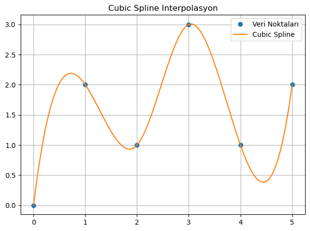
1. 📌 Cubic Spline Interpolasyon¶

Veri noktaları arasında pürüzsüz geçişler sağlayan kübik spline yöntemi.

from scipy.interpolate import CubicSpline
import numpy as np
import matplotlib.pyplot as plt

x = np.array([0, 1, 2, 3, 4, 5])
y = np.array([0, 2, 1, 3, 1, 2])

cs = CubicSpline(x, y)
x_new = np.linspace(x.min(), x.max(), 300)
y_new = cs(x_new)

plt.plot(x, y, 'o', label='Veri Noktaları')
plt.plot(x_new, y_new, '-', label='Cubic Spline')
plt.title('Cubic Spline Interpolasyon')
plt.legend()
plt.grid(True)
plt.tight_layout()
plt.show()

Cubic Spline

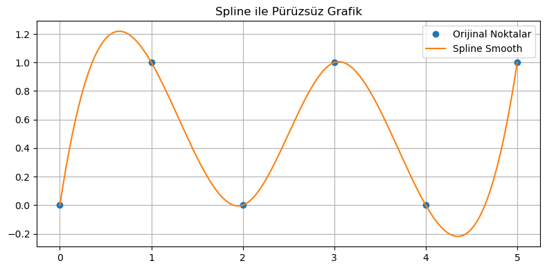
2. 📌 make_interp_spline (Spline Smooth)¶

import numpy as np
import matplotlib.pyplot as plt
from scipy.interpolate import make_interp_spline

# Veri
x = np.array([0, 1, 2, 3, 4, 5])
y = np.array([0, 1, 0, 1, 0, 1])

# Daha sık aralıkla yeni x oluştur
x_new = np.linspace(x.min(), x.max(), 300)

# Smooth fonksiyon oluştur
spl = make_interp_spline(x, y, k=3)  # k=3 → cubic spline
y_smooth = spl(x_new)

# Grafik
plt.figure(figsize=(8, 4))
plt.plot(x, y, 'o', label="Orijinal Noktalar")
plt.plot(x_new, y_smooth, '-', label="Spline Smooth")
plt.legend()
plt.title("Spline ile Pürüzsüz Grafik")
plt.grid(True)
plt.tight_layout()
plt.show()

make_interp_spline

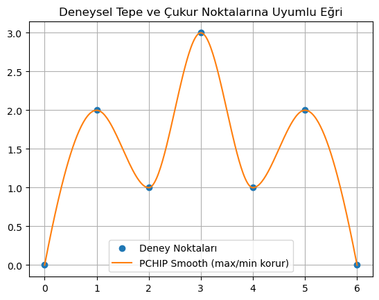
3. 📌 PCHIP Interpolasyon (Tepe & Çukur Noktaları Korur)¶

from scipy.interpolate import PchipInterpolator
import matplotlib.pyplot as plt
import numpy as np

x = np.array([0, 1, 2, 3, 4, 5, 6])
y = np.array([0, 2, 1, 3, 1, 2, 0])  # Deneysel maksimum-minimum noktalar dahil

x_new = np.linspace(x.min(), x.max(), 300)
pchip = PchipInterpolator(x, y)
y_new = pchip(x_new)

plt.plot(x, y, 'o', label='Deney Noktaları')
plt.plot(x_new, y_new, '-', label='PCHIP Smooth (max/min korur)')
plt.legend()
plt.grid(True)
plt.title("Deneysel Tepe ve Çukur Noktalarına Uyumlu Eğri")
plt.show()

PCHIP

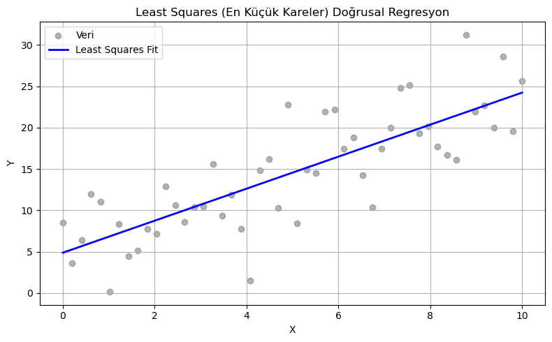
4. 📌 Least Squares Doğrusal Regresyon¶

import numpy as np
import matplotlib.pyplot as plt

# Rastgele doğrusal veri
np.random.seed(0)
x = np.linspace(0, 10, 50)
y_true = 2.5 * x + 1.5
y = y_true + np.random.normal(scale=4, size=x.shape)

# Least Squares ile doğrusal regresyon
coeffs = np.polyfit(x, y, 1)  # 1. dereceden polinom
y_fit = np.polyval(coeffs, x)

# Grafik
plt.figure(figsize=(8, 5))
plt.scatter(x, y, color='gray', label='Veri', alpha=0.6)
plt.plot(x, y_fit, color='blue', linewidth=2, label='Least Squares Fit')
plt.title("Least Squares (En Küçük Kareler) Doğrusal Regresyon")
plt.xlabel("X")
plt.ylabel("Y")
plt.legend()
plt.grid(True)
plt.tight_layout()
plt.show()

print(f"Eğim (m): {coeffs[0]:.4f}, Y-kesişim (b): {coeffs[1]:.4f}")

Least Squares

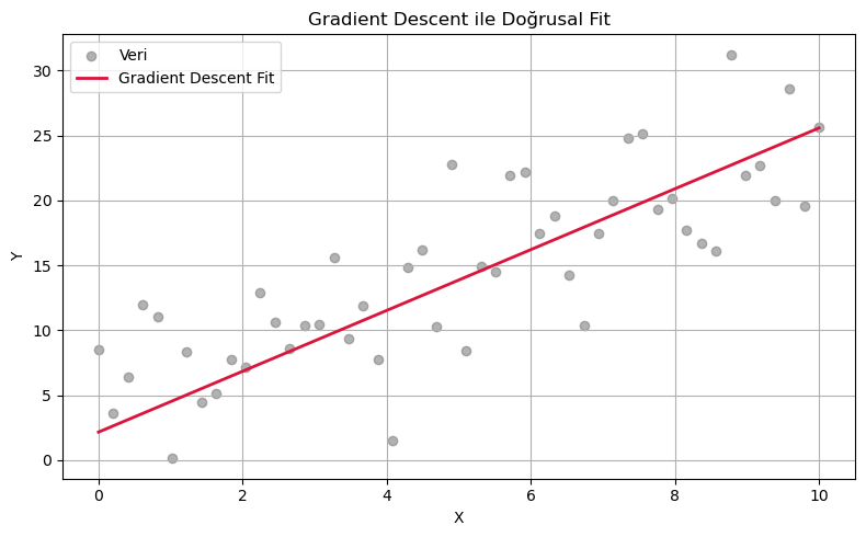
5. 📌 Gradient Descent ile Doğrusal Regresyon¶

import numpy as np
import matplotlib.pyplot as plt

# Veri
np.random.seed(0)
x = np.linspace(0, 10, 50)
y_true = 2.5 * x + 1.5
y = y_true + np.random.normal(scale=4, size=x.shape)

# Parametre başlangıcı
m, b = 0.0, 0.0
learning_rate = 0.001
epochs = 1000

# Gradient Descent
for _ in range(epochs):
    y_pred = m * x + b
    error = y_pred - y
    m_grad = (2 / len(x)) * np.dot(error, x)
    b_grad = (2 / len(x)) * np.sum(error)
    m -= learning_rate * m_grad
    b -= learning_rate * b_grad

y_fit = m * x + b

# Grafik
plt.figure(figsize=(8, 5))
plt.scatter(x, y, color='gray', label='Veri', alpha=0.6)
plt.plot(x, y_fit, color='crimson', linewidth=2, label='Gradient Descent Fit')
plt.title("Gradient Descent ile Doğrusal Fit")
plt.xlabel("X")
plt.ylabel("Y")
plt.legend()
plt.grid(True)
plt.tight_layout()
plt.show()

print(f"Eğim (m): {m:.4f}, Y-kesişim (b): {b:.4f}")

Gradient Descent

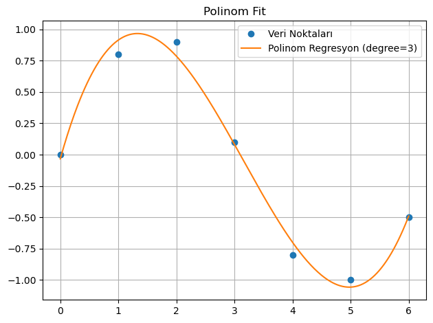
6. 📌 Polinom (polyfit) Regresyon¶

import numpy as np
import matplotlib.pyplot as plt

# Örnek veri
x = np.array([0, 1, 2, 3, 4, 5, 6])
y = np.array([0, 0.8, 0.9, 0.1, -0.8, -1.0, -0.5])

# İnterpolasyon için daha sık x noktaları oluştur
x_new = np.linspace(x.min(), x.max(), 300)

# 3. dereceden polinom fit
z = np.polyfit(x, y, deg=3)
p = np.poly1d(z)
y_fit = p(x_new)

# Grafik
plt.plot(x, y, 'o', label='Veri Noktaları')
plt.plot(x_new, y_fit, '-', label='Polinom Regresyon (degree=3)')
plt.title('Polinom Fit')
plt.legend()
plt.grid(True)
plt.tight_layout()
plt.show()

Polinom (polyfit)

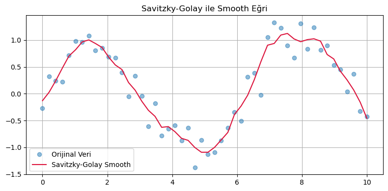
7. 📌 Savitzky-Golay Regresyon¶

import numpy as np
import matplotlib.pyplot as plt
from scipy.signal import savgol_filter

# Örnek veri (daha yoğun)
x = np.linspace(0, 10, 50)
y = np.sin(x) + 0.3 * np.random.randn(50)  # Gürültülü veri

# Smooth y
y_smooth = savgol_filter(y, window_length=9, polyorder=3)

# Grafik
plt.figure(figsize=(8, 4))
plt.plot(x, y, 'o', label="Orijinal Veri", alpha=0.5)
plt.plot(x, y_smooth, '-', label="Savitzky-Golay Smooth", color='crimson')
plt.legend()
plt.grid(True)
plt.title("Savitzky-Golay ile Smooth Eğri")
plt.tight_layout()
plt.show()

Savitzky-Golay

📎 Appendix¶

Interpolasyon ve Regresyon HTML